Real-Time 3D Rendering in XPL0
By Boreal
Great! You're ready for some more XPL0 programming.
This is a continuation of "Creating Demos in XPL0." Like the previous
article, this is inspired by Polaris's tutorials in Hugi 31. Here we'll
build upon the 3D wireframe introduced in his Tutorial #7. We'll use the
classic torus as our subject, and cook up a recipe for turning it into a
donut.
All the code and executables are in the bonus pack in torusxpl.zip. You need
to run the programs to appreciate the speed that the images are drawn.
They run under DOS and most versions of Windows. The programs are
terminated by pressing the Esc key. Some depend on the file texture.bmp,
which prevents them from being run directly from the zip file under
Windows. You must extract those programs into a folder.
Coordinates
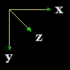 You'll get hopelessly confused if you don't know which way is which. The
examples here use a right-handed coordinate system with the Z axis going
into the screen. Other graphic systems, such as DirectX and OpenGL, use
different conventions. It isn't important which convention you use as
long as you stick to it throughout a program.
You'll get hopelessly confused if you don't know which way is which. The
examples here use a right-handed coordinate system with the Z axis going
into the screen. Other graphic systems, such as DirectX and OpenGL, use
different conventions. It isn't important which convention you use as
long as you stick to it throughout a program.
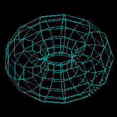
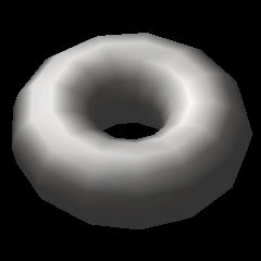
Torus1
The first example is very short just to get the ball rolling - or rather
the torus tumbling.
The SetUp procedure (see below) uses some sines and cosines to define a
series of points on the surface of a torus. The Draw procedure connects
these points with a network of lines to form a wireframe image. The
Rotate procedure rotates these points about the X, Y and Z axes. They are
moved a small amount each time the procedure is called.
The Rotate procedure is probably the most mysterious of the bunch. It
uses difference equations to approximate sines and cosines of small
angles. Sines and cosines, of course, are the standard way to rotate a
point in analytic geometry. The advantage of the difference equations is
they are simple and fast compared to floating-point sines and cosines.
This was important once upon a time, but not so much now with the
capabilities of modern processors. There is however a problem with this
technique. It accumulates errors. If you run Torus1 for a minute or two,
you'll see something interesting.
Take a glance at the code to get a feel for what it's doing. (This will
be the last complete source listing you're forced to look at. The source
for every example is in the bonus pack.)
include c:\cxpl\codesi;         \intrinsic code definitions

def     C1=130, C2=80;  \determine speed of rotation (larger values are slower)
def     TorR1 = 10000.0,\distance from the center of the hole in the middle
                        \ to the center of the eatable tube-shaped part
        TorR2 = 6000.0; \the distance from the center of the eatable tube-
                        \ shaped part to the frosting on top
def     Sectors = 13,   \number of slices of the torus (tubes)
        Sections = 13;  \number of slices of a sector (patches)
int     TorX(Sectors+1,Sections+1),     \coordinates of vertexes approximating
        TorY(Sectors+1,Sections+1),     \ a torus
        TorZ(Sectors+1,Sections+1);


proc    VSync;                  \Wait for vertical retrace to begin
begin
while PIn($3DA,0) & $08 do [];  \wait for vertical retrace signal to go away
repeat until PIn($3DA,0) & $08; \wait for vertical retrace
end;    \VSync


proc    Rotate;                 \Rotate the torus
int     I, J;
begin
for I:= 0, Sectors do
    for J:= 0, Sections do
        begin
        TorX(I,J):= TorX(I,J) + TorY(I,J)/C1;
        TorY(I,J):= TorY(I,J) - TorX(I,J)/C1;
        TorY(I,J):= TorY(I,J) + TorZ(I,J)/C2;
        TorZ(I,J):= TorZ(I,J) - TorY(I,J)/C2;
        end;
end;    \Rotate


proc    Draw;                   \Draw the torus
int     I, J;
def     CX=640/2, CY=480/2,     \coordinates of center of screen
        Scale=80,               \de-magnification factor
        Color=3;                \cyan
begin
for J:= 0, Sections-1 do
        begin
        Move(TorX(0,J)/Scale+CX, TorY(0,J)/Scale+CY);
        for I:= 1, Sectors do
                Line(TorX(I,J)/Scale+CX, TorY(I,J)/Scale+CY, Color);
        end;
for I:= 0, Sectors-1 do
        begin
        Move(TorX(I,0)/Scale+CX, TorY(I,0)/Scale+CY);
        for J:= 1, Sections do
                Line(TorX(I,J)/Scale+CX, TorY(I,J)/Scale+CY, Color);
        end;
end;    \Draw


proc    SetUp;
\Find the coordinates of the vertexes of facets that approximate a torus.
\Chop the surface of the torus up into facets (polygons). To simplify later
\ calculations, the last coordinates duplicate the first coordinates. The
\ torus is initially in the X,Y plane (like a donut floating in hot grease).
\Outputs: TorX, TorY, TorZ.
int     I, J;
real    A,              \angular increments about the hole in the center
        B,              \angular increments about the center of the tube
        SA, CA, SB, CB; \sines and cosines of A and B
def     Pi2 = 2.0 * 3.14159265358979323846;
begin
for I:= 0, Sectors do
        begin
        A:= Float(I) / Float(Sectors) * Pi2;
        SA:= Sin(A);   CA:= Cos(A);
        for J:= 0, Sections do
                begin
                B:= Float(J) / Float(Sections) * Pi2;
                SB:= Sin(B);   CB:= Cos(B);
                TorX(I,J):= Fix((TorR1 + TorR2*CB) * CA);
                TorY(I,J):= Fix((TorR1 + TorR2*CB) * SA);
                TorZ(I,J):= Fix(TorR2 * SB);
                end;
        end;
end;    \SetUp


begin   \Main
SetVid($12);                    \640x480x16 graphics
SetUp;
loop    begin
        Clear;                  \erase screen
        Draw;                   \draw the torus
        Rotate;                 \rotate the torus for the next frame
        if ChkKey then quit;    \terminate program if any keystroke
        VSync;                  \wait for vertical blank
        VSync;                  \wait again to provide a 30th second delay
        end;
OpenI(0);                       \eat the keystroke
SetVid(3);                      \restore normal text mode
end;    \Main
Torus2
 The second version of our program elaborates on Torus1 by making it
interactive. It uses the mouse and keyboard to manipulate the image. This
also solves the problem of accumulating errors in the rotation
calculations. You may have noticed that these eventually caused the torus
to get bent all out of shape.
The second version of our program elaborates on Torus1 by making it
interactive. It uses the mouse and keyboard to manipulate the image. This
also solves the problem of accumulating errors in the rotation
calculations. You may have noticed that these eventually caused the torus
to get bent all out of shape.
The new procedures RotateTorus and Rotate use the mouse to rotate the
image. RotateTorus gets angles from the mouse and uses them to rotate a
reference frame by calling Rotate. Rotate uses sine and cosine
calculations to rotate the reference frame about the X, Y and Z axes. The
code shows the standard matrix notation that is typically used. A matrix
multiply is applied to each point (vertex) in the torus to align it with
the rotated reference frame.
The rest of the code is relatively easy to understand. It uses keyboard
commands to adjust the number of sectors and sections in the torus.
GetKey and CallInt are simple routines that facilitate calls to BIOS. If
you hold down the arrow keys, you can get a well-rounded torus.
proc Rotate(V, R, P, W); \3D rotate vector V
real V, \3D vector is 3-element array with X, Y and Z components
R, P, W; \Roll, Pitch and yaW (radians)
real X, Y, Z, SW, SP, SR, CW, CP, CR, T;
begin
X:= V(0); Y:= V(1); Z:= V(2); \get vector components
SR:= Sin(R); SP:= Sin(P); SW:= Sin(W);
CR:= Cos(R); CP:= Cos(P); CW:= Cos(W);
\Rotate about X axis (Roll):
T:= Y*CR - Z*SR; \ � �
Z:= Z*CR + Y*SR; \ �1 0 0 �
Y:= T; \ [X Y Z]:= [X Y Z] * �0 CR SR�
\ �0 -SR CR�
\ � �
\Rotate about Y axis (Pitch):
T:= X*CP + Z*SP; \ � �
Z:= Z*CP - X*SP; \ �CP 0 -SP�
X:= T; \ [X Y Z]:= [X Y Z] * �0 1 0 �
\ �SP 0 CP�
\ � �
\Rotate about Z axis (yaW):
T:= X*CW - Y*SW; \ � �
Y:= Y*CW + X*SW; \ � CW SW 0 �
X:= T; \ [X Y Z]:= [X Y Z] * �-SW CW 0 �
\ � 0 0 1 �
\ � �
V(0):= X; V(1):= Y; V(2):= Z; \return values
end; \Rotate
proc CrossProd(V1, V2, V3); \Calculate the cross product of two 3D vectors
real V1, V2, V3; \V3:= V1 x V2
def X, Y, Z; \dimensions
begin
V3(X):= V1(Y)*V2(Z) - V1(Z)*V2(Y);
V3(Y):= V1(Z)*V2(X) - V1(X)*V2(Z);
V3(Z):= V1(X)*V2(Y) - V1(Y)*V2(X);
end; \CrossProd
proc RotateTorus; \Rotate torus by moving the mouse
\Inputs: Sectors, Sections, TorX, TorY, TorZ.
\Outputs: RTorX, RTorY.
int I, J; \indexes
real AngX, AngY, AngZ, \rotation angle about indicated axis (radians)
Rxx, Rxy, Rxz, \rotation matrix
Ryx, Ryy, Ryz,
Rzx, Rzy, Rzz;
def X, Y, Z; \dimensions
begin
CallInt($33, $0B); \read mouse motion counters
\Mouse X motion rotates object about Y axis
AngY:= Float(-CpuReg(2)) / 500.0;
\Mouse Y motion rotates object about X axis
AngX:= Float(CpuReg(3)) / 500.0;
AngZ:= 0.0;
\STEP 1:
\Rotate reference frame according to changes in mouse position.
\Independently rotating P1 and P2 can cause them to drift relative to
\ each other, but the amount of drift is insignificant because reals are
\ accurately calculated to 16 decimal places.
Rotate(Ref1, AngX, AngY, AngZ);
Rotate(Ref2, AngX, AngY, AngZ);
CrossProd(Ref1, Ref2, Ref3); \Ref3:= Ref1 x Ref2
\STEP 2:
\Rotate each vertex in the object so that it aligns with the reference frame:
\Replace subscripted variables for efficiency and neatness:
Rxx:= Ref1(X); Rxy:= Ref1(Y); Rxz:= Ref1(Z);
Ryx:= Ref2(X); Ryy:= Ref2(Y); Ryz:= Ref2(Z);
Rzx:= Ref3(X); Rzy:= Ref3(Y); Rzz:= Ref3(Z);
\This multiplies each point at its initial position (Po) by the rotation
\ matrix to get the rotated position
\ � �
\ � � � � � Rxx Rxy Rxz �
\ � Px Py Pz � = � Pxo Pyo Pzo � * � Ryx Ryy Ryz �
\ � � � � � Rzx Rzy Rzz �
\ � �
\
for I:= 0, Sectors do \for all of the sectors+1...
for J:= 0, Sections do \for all of the sections+1...
begin \(end points duplicate first points)
RTorX(I,J):= Fix((TorX(I,J)*Rxx + TorY(I,J)*Ryx + TorZ(I,J)*Rzx)*Scale);
RTorY(I,J):= Fix((TorX(I,J)*Rxy + TorY(I,J)*Ryy + TorZ(I,J)*Rzy)*Scale);
end;
end; \RotateTorus
Torus3
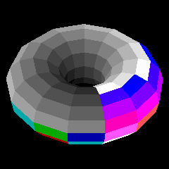 This version of our Torus program increases realism by replacing the
wireframe with solid surfaces. To make the surfaces colorful, and to draw
them quickly, we take advantage of VESA graphics and 32-bit XPL0.
This version of our Torus program increases realism by replacing the
wireframe with solid surfaces. To make the surfaces colorful, and to draw
them quickly, we take advantage of VESA graphics and 32-bit XPL0.
The major changes to the code are a DrawPoly procedure and a couple sort
procedures.
DrawPoly draws a filled polygon, or in our case, a 4-sided figure called
a "quad." Instead of drawing directly on the screen, DrawPoly draws onto
a buffer named Image. This buffer is then copied to the screen using the
Paint intrinsic. This technique eliminates the flicker noticeable in
Torus1 and Torus2.
With the wireframe models it didn't matter which order the lines were
drawn, but with solid surfaces it's essential that the back surfaces
never obscure the front ones. This is where the sort routines come in.
The surfaces are sorted according to their distance from the viewer. In
other words, they are sorted according to their Z-axis positions, or
depth. DrawTorus then draws the surfaces starting with the one with the
greatest Z position and works its way toward the front. This technique is
known as the Painter's Algorithm. The Image buffer not only eliminates
flicker, but it also prevents showing all the overpainting that's being
done.
When you look at the code you'll see other minor changes. WExtend is used
to sign-extend the 16-bit values, returned by DOS and BIOS, to the 32-bit
values used by XPL0. Also the array names are streamlined. For instance
TorX, TorY and TorZ are collapsed into a single array with an extra
dimension added for the X, Y and Z axes.
Torus4
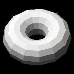 This version shines some light on the subject, which adds another step in
realism.
This version shines some light on the subject, which adds another step in
realism.
In Torus3 light was emitted by colored facets. Now, in Torus4 the facets
are illuminated with two kinds of light: directional and ambient.
Directional light is like the light from the sun. Ambient light is the
kind of light that gets scattered around inside a room. Both are
necessary.
If only ambient light is used then all the facets look identical and
blend together. If only directional light is used then the facets facing
away from the light are invisible. In the program if you adjust Ambient
all the way up and down, you'll see these effects.
The amount of light that reflects from a rough, non-shiny surface depends
on the direction the surface is facing. If it points directly toward a
source of light then it reflects the maximum amount. If it's tilted away
from the light then the intensity of the reflected light is diminished
depending on the angle of tilt. The amount of reflected light is
determined by Lambert's Law, which states that the intensity is
proportional to the cosine of the angle between the direction of the
surface and the direction of the light source. The intensity does not
depend on the direction of the viewer because the reflected light is
equally scattered in all directions.
Vectors perpendicular to each surface, called "normal vectors," are added
to the code to measure angles of tilt. The dot-product turns out to be a
simple way to calculate the cosine of the angle between the normal vector
and the direction of the light, which is also a vector.
Normal vectors serve another purpose. A surface that faces away from the
viewer will have a positive Z component in its normal vector. Torus4
exploits this to eliminate drawing these surfaces; instead of merely
painting over them, as was done in Torus3. This not only speeds things
up, but it also fixes a little glitch in Torus3 when there are only 3
sectors and 3 sections. (It's not always easy to determine which polygon
is behind another.)
Speed is something that needs to be kept in mind when doing animation.
Thus "Frames/second" is added to the display. This shows the number of
times the screen gets redrawn each second. You can see how the various
adjustments affect speed. For instance, lots of facets slow things
down.
Torus5
 This version smoothes the surface of the torus without reverting to lots
of facets by using a technique called Gouraud shading. This varies the
brightness of the reflected light across the face of a facet.
This version smoothes the surface of the torus without reverting to lots
of facets by using a technique called Gouraud shading. This varies the
brightness of the reflected light across the face of a facet.
To accomplish this an additional set of normal vectors are added at the
vertices. These are the average of the adjacent surface normals that were
introduced in Torus4. Lambert's Law is applied to give the intensity of
the reflected light at each vertex, instead of at each face, and this
provides a color for the DrawPoly procedure.
DrawPoly is modified to interpolate color between vertices. First it
interpolates the color along the edges of the polygon (in the procedure
BuildLine). Then it interpolates the color along the horizontal scan
lines that fill the area between the edges. The result is a smoothly
changing gradient of color across the surface of the polygon.
Interpolation only adds a small amount of overhead to the time-critical
innermost loops of the code. The result is that curved surfaces can
quickly be smoothly shaded without resorting to lots of facets.
Here are some speed comparisons on two computers: a Duron 850 and an
Athlon 2400+ with an nVidia card. The number of frames per second are
shown for the reset condition (13 sectors, 13 sections, straight-on
view) and for the extreme condition (63 sectors, 63 sections).
                    Duron                   Athlon
                13x13    63x63          13x13    63x63
                -------------           --------------
        Torus4   66 fps   32            117 fps   67
        Torus5   59       23            106       52
Pan and zoom are also added to this version. To move the torus about the
screen, hold the right mouse button down. To magnify it, hold both
buttons (or the center button) and move the mouse forward. (Can you turn
it inside out?)
Pan and zoom are simple modifications to the RotateTorus procedure.
Making DrawPoly clip the image at the edge of the screen without
distorting the shading is a little more involved.
Torus6
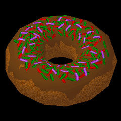 This version takes a giant leap toward realism by converting the torus
into an actual donut - complete with sprinkles!
This version takes a giant leap toward realism by converting the torus
into an actual donut - complete with sprinkles!
"Texture mapping" is the magic new ingredient. This applies the image in
the file texture.bmp onto the surface of the torus. It uses the same
interpolation idea as for Gouraud shading. In addition to interpolating
light intensity, DrawPoly now interpolates horizontal and vertical steps
through the texture image. The colors of the pixels that get selected
from this image are used to plot the pixels that fill the polygons
displayed on the screen.
The color selected is not plotted directly, but instead its brightness is
adjusted so that the donut gets shaded, giving it a 3D look. To keep the
code fast this brightness adjustment is gotten from a color look-up table
(CLUT), which is set up by the procedure MakeCLUT. Given a color and
brightness, the table provides a shaded color.
Gouraud shading can be turned on and off using the G key. This lets you
see the tradeoff in speed and appearance for various numbers of facets.
Notice that while Gouraud shading is effective in smoothing (especially
the underside of the donut) it does nothing to smooth the edges of the
silhouette. Gouraud shading definitely looks better than flat shading
when there are only 13x13 facets; but when there are 63x63 facets, it's
little, if any, improvement. However, 63x63 facets take a long time to
render.
Torus7
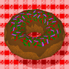 Alas, a shadow has finally fallen on this project.
This version adds two new procedures: DrawBkgnd provides a background
image, so the shadow has something to fall upon; and DrawShadow provides
the shadow.
DrawBkgnd does a series of calls to DrawPoly to provide a checkered
tablecloth. It's drawn in the X-Y plane at Z=0.
The star of this version is DrawShadow, and its magic can simply be
stated like this:
Shadow = Torus - dist*Light
Shadow, Torus and Light are 3D vectors. Light is a unit vector that when
multiplied by the (1D) scalar "dist" gives a vector from a point on the
torus to the corresponding point in its shadow.
Since the Z component of Shadow is 0, equations for the X and Y
components can easily be derived.
        Shadow(Z) = 0 = Torus(Z) - dist*Light(Z)
Thus:
        dist = Torus(Z)/Light(Z)
Substituting this expression for "dist" in the equations for the X and Y
components gives:
        Shadow(X) = Torus(X) - Torus(Z)/Light(Z)*Light(X)
        Shadow(Y) = Torus(Y) - Torus(Z)/Light(Z)*Light(Y)
Shadow(X) and Shadow(Y) are the coordinates that DrawPoly needs to draw
the shadows on the tablecloth for each of the polygons that make up the
torus.
Wrap-up
This is difficult to follow, I know. At least you have the highlights (no
pun intended) and can dig out the details in the code if you desire.
Unlike with DirectX or even OpenGL everything is there. Once you plow
through that, you'll understand everything - or at least enough to start
building your own 3D engine.
Good luck!
-
Boreal (aka: Loren Blaney)
loren_blaney@idcomm.com